DyFe$_2$

In common with all the samples studied in this chapter at room temperature the 750Å DyFe$_{2}$ sample needs a minimum of four components to be fitted properly. Figure 6.3 shows the spectra for all of the thin film samples studied in zero applied field. Four inequivalent iron sites confirm the easy axis is not along any of the high symmetry directions expected in bulk systems.

Figure 6.3: Comparison of spectra of DyFe$_{2}$, YFe$_{2}$ and HoFe$_{2}$ thin films at room temperature under zero applied field.

The best fit parameters for the DyFe$_{2}$ samples in zero applied field are shown in Table 6.1 for fits assuming $\left[\bar{2}41\right]$ or $\left[\bar{3}51\right]$ easy axis directions with values calculated according to the dipole hyperfine field analysis in Section 6.2.1.

Table: Final fit parameters for 750Å DyFe$_{2}$ sample assuming $\left[\bar{2}41\right]$ or $\left[\bar{3}51\right]$ easy axis in zero applied field.

$$\left[\bar{2}41\right] \left[\bar{3}51\right]$$

$$H_{S}=205\pm2\ensuremath{\unskip\,\mathrm{kG}} H_{S}=205\pm5\ensuremath{\unskip\,\mathrm{kG}}$$

$$H_{D}=15\pm4\ensuremath{\unskip\,\mathrm{kG}} H_{D}=17\pm7\ensuremath{\unskip\,\mathrm{kG}}$$

$$\chi^{2}=2.05 \chi^{2}=2.06$$

Site IS QS Field IS QS Field

$$(\nicefrac{mm}{s}) (\nicefrac{mm}{s}) (\nicefrac{mm}{s}) (\nicefrac{mm}{s})$$ (kG) (kG)

$$[111] -0.1 -0.0604 198.8 -0.1 -0.0935 199.7$$

$$[11\bar{1}] -0.1 -0.1387 182.5 -0.1 -0.1432 182.5$$

$$[\bar{1}11] -0.1 +0.2191 209.1 -0.1 +0.2167 208.8$$

$$[1\bar{1}1] -0.1 +0.0644 205.7 -0.1 +0.0949 204.8$$

The isomer shift values (IS) are fixed to be equal for all components but free to vary as a whole. The IS value of $-0.1\ensuremath{\unskip\,\mathrm{\nicefrac{mm}{s}}}$ is consistent with those reported for bulk samples[32]. The quadrupole splitting is fixed and its value is calculated using the analysis outlined in Section 6.2.1.

The hyperfine fields are initially fixed according to the values calculated from $\boldsymbol{H}_{S}$ and $\boldsymbol{H}_{D}$ and then allowed to vary. The theoretical values do not give satisfactory fits and are allowed to freely vary (with the quadrupole splitting remaining constant). Iteratively varying $H_{S}$ and $H_{D}$ to account for the difference is prohibitively time consuming as it is not an automated process: there is no way to automatically transfer the parameters from the dipolar field analysis into the Mössbauer fitting routines. The spread in values is from the different angle that the axis of symmetry at each iron site makes with the magnetic easy axis, and hence the dipolar field contribution is different.

The values of $H_{S}$ and $H_{D}$ (Table 6.1) obtained are consistent with those found for bulk samples.[27] There is no significant difference between the fits for $\left[\bar{2}41\right]$ and $\left[\bar{3}51\right]$ easy axes either in the quality of the fitting of theory to the spectrum or in the comparison of the derived hyperfine field values with those from other studies.

A spectrum was recorded under an in plane applied field, ($H_{0}$ in Equation 2.17) of $2.5\ensuremath{\unskip\,\mathrm{kOe}}$. This spectrum is compared to the zero applied field spectrum in Figure 6.4 and the fit parameters compared in Table 6.2. The fitting parameters do not have any particular easy axis applied. The Isomer Shifts and relative line intensities are fixed to be equal for all sites but free to vary.

Figure: 750Å DyFe$_{2}$ thin film under $0\ensuremath{\unskip\,\mathrm{kOe}}$ and $2.5\ensuremath{\unskip\,\mathrm{kOe}}$ in plane applied magnetic fields.

Table: Final fit parameters for the 750Å DyFe$_{2}$ sample in $0\ensuremath{\unskip\,\mathrm{kOe}}$ or $2.5\ensuremath{\unskip\,\mathrm{kOe}}$ in plane applied field. No particular easy axis is applied to the fitting parameters. The average angle is relative to the sample plane.

$$0\ensuremath{\unskip\,\mathrm{kOe}} 2.5\ensuremath{\unskip\,\mathrm{kOe}}$$

$$\chi^{2}=2.53 \chi^{2}=1.91$$

Site IS QS Field Angle IS QS Field Angle

$$(\nicefrac{mm}{s}) (\nicefrac{mm}{s}) ^{\circ} (\nicefrac{mm}{s}) (\nicefrac{mm}{s}) ^{\circ}$$ (kG) (kG)

$$1 -0.10 -0.24 186.6 -0.09 -0.32 185.2$$ 23.3 23.1

$$2 -0.10 +0.12 200.6 -0.09 +0.19 197.0$$ 23.3 23.1

$$3 -0.10 +0.22 209.2 -0.09 +0.16 208.6$$ 23.3 23.1

$$4 -0.10 -0.01 200.2 -0.09 -0.01 197.1$$ 23.3 23.1

The change in average angle of the spin moments under applied field is $0.2^{\circ}$. The two spectra were not recorded sequentially and thus this change in angle is well within the experimental error of the relative angular positioning of the source and sample, taken to be $2^{\circ}$.

The change in the average hyperfine field^6.2 due to the applied field is $-2.35\ensuremath{\unskip\,\mathrm{kG}}$. The negative change in the hyperfine field indicates the iron moments being parallel to $H_{0}$: the hyperfine field lies antiparallel to the magnetic moment. It was expected that the hyperfine fields would increase as the dysprosium moments, being significantly larger than the iron moments, would tend to align parallel with an applied field. Through the antiferromagnetic coupling the iron moments would then be lying antiparallel to the applied field.

To explain this there are competing effects in the sample under an applied field from the sample and the seed layer. Although the signal from the seed layer underneath the $750\ensuremath{\unskip\,\mathrm{\AA{}}}$ sample layer produces at most a $15\%$ background contribution to the spectrum (using the theory outlined in Section 2.5.2), the seed layer can influence the moment orientation of the sample layer. In this bilayer arrangement a magnetic exchange-spring can be produced, where the moments in the soft magnetic seed layer twist at their free end whilst being pinned by the hard magnetic sample layer.

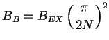
The onset of this exchange spring under an applied field is governed by a critical bending field $B_{B}$. For a bilayer this is related to the exchange field, $B_{EX}$, by the relation

$$B_{B} = B_{EX}\left( \frac{\pi}{2N} \right)^{2}$$ (6.11)

where $N$ is the number of monolayers in the soft magnetic layer.[33] The exchange spring also penetrates into the hard magnetic layer, with the extent determined by the strength of the applied field and the axial anisotropy of the hard magnetic layer. Using the conditions cited in Reference bowden_00 for DyFe$_2$/YFe$_2$, an iron-iron exchange field $B_{EX}=6000\ensuremath{\unskip\,\mathrm{kOe}}$ and $N=114$ gives a bending field $B_{B}=0.7\ensuremath{\unskip\,\mathrm{kOe}}$. Our applied field of $2.5\ensuremath{\unskip\,\mathrm{kOe}}$ is thus sufficient to produce an exchange spring.

The applied field should, however, be far too small to overcome the single ion anisotropy of the DyFe$_2$ thin film (fields an order of magnitude greater than used in these measurements were used in Reference bowden_00 without overcoming the anisotropy of the hard magnetic pinning layer). Whilst a small portion at the interface with the YFe$_2$ seed layer would be rotated somewhat along the applied field direction it is expected that the majority of the upper sample layer (also from which the majority of the CEMS signal is obtained) would be unperturbed. A sample oriented with the Dy moments antiparallel to the applied field would give the observed results. The arrangement of the sample within the spectrometer was not recorded, however, so this is currently conjecture.

DyFe$_{2}$, in bulk, has an easy axis that lies along one of the $\langle100\rangle$ directions. As the sample geometry includes the $\left[001\right]$ direction in the plane of the sample, also favoured by the shape anisotropy of a thin film, the magneto-elastic energy must be substantial to produce an easy axis so far out of plane. This direction is seemingly unperturbed by the application of a $2.5\ensuremath{\unskip\,\mathrm{kOe}}$ field, also trying to force the moments into the plane of the sample. Without higher field or temperature measurements (both of which are impossible with the CEMS equipment) an absolute value of $E_{me}$ cannot be calculated but the data point to it being of at least the same order as the magnetocrystalline and shape anisotropy energies combined.