Next: DyFe Up: RFe Thin Films Previous: RFe Thin Films Contents
A particularly important parameter to extract from the spectra is the direction of the magnetic easy axis. This is well known in bulk RFe![]() intermetallics[24] but has been shown to not be along any expected high-symmetry axis in thin films at room temperature[29,30]. Mössbauer spectroscopy is particularly sensitive to the orientation of magnetic moments at a particular site, either through the angular dependency of the dipolar hyperfine field (Equation 2.20) or from the relative line intensities (Equation 2.24). The latter is often much more pronounced and so easy to obtain reliable information from.
intermetallics[24] but has been shown to not be along any expected high-symmetry axis in thin films at room temperature[29,30]. Mössbauer spectroscopy is particularly sensitive to the orientation of magnetic moments at a particular site, either through the angular dependency of the dipolar hyperfine field (Equation 2.20) or from the relative line intensities (Equation 2.24). The latter is often much more pronounced and so easy to obtain reliable information from.
Previous work on single-crystal RFe![]() thin films by V. Oderno et al[29] showed that the easy direction was
thin films by V. Oderno et al[29] showed that the easy direction was
![]() at
at
![]() but was a direction of low symmetry at room temperature. Their best fits were for those assuming an easy magnetic axis of
but was a direction of low symmetry at room temperature. Their best fits were for those assuming an easy magnetic axis of
![]() , with
, with
![]() ,
,
![]() ,
,
![]() and
and
![]() being the most likely as they were closest to the angle displayed by their Mössbauer spectra. Subsequent experiments by Mougin et al[30] again showed the difference in easy axis at
being the most likely as they were closest to the angle displayed by their Mössbauer spectra. Subsequent experiments by Mougin et al[30] again showed the difference in easy axis at
![]() and room temperature. Their analysis indicated an easy axis along
and room temperature. Their analysis indicated an easy axis along
![]() directions, with the most likely being
directions, with the most likely being
![]() . Consequently our analysis starts with the assumption of a
. Consequently our analysis starts with the assumption of a
![]() or
or
![]() easy axis at room temperature.
easy axis at room temperature.
However, the proposed easy axes of
![]() or
or
![]() both have a high level of degeneracy in a cubic system, corresponding to 24 different directions. These samples are conceived as single-crystal, thus a given axis such as
both have a high level of degeneracy in a cubic system, corresponding to 24 different directions. These samples are conceived as single-crystal, thus a given axis such as
![]() denotes a unique axis in the sample. However, there will be magnetic domains in which the magnetisation direction, while linked to an equivalent direction of
denotes a unique axis in the sample. However, there will be magnetic domains in which the magnetisation direction, while linked to an equivalent direction of
![]() , does not define a unique direction in the sample. Thus the Mössbauer spectrum will display the relative directions of
, does not define a unique direction in the sample. Thus the Mössbauer spectrum will display the relative directions of ![]() and
and ![]() through line positions but will not give reliable information through relative line intensities as these can be affected by different magnetic domain patterns which can be affected by sample history. In the absence of a training field there are still physical characteristics which favour particular directions. The shape anisotropy of the sample will favour moments that are more in plane and this is corroborated by the average angle obtained from the line intensities of 21
through line positions but will not give reliable information through relative line intensities as these can be affected by different magnetic domain patterns which can be affected by sample history. In the absence of a training field there are still physical characteristics which favour particular directions. The shape anisotropy of the sample will favour moments that are more in plane and this is corroborated by the average angle obtained from the line intensities of 21![]() to the sample plane (for DyFe
to the sample plane (for DyFe![]() ). This does, however, still leave at least four non-equivalent directions and with no direct evidence of their relative populations.[29]
). This does, however, still leave at least four non-equivalent directions and with no direct evidence of their relative populations.[29]
In interpreting the line positions of the Mössbauer spectra with high accuracy it is necessary to consider the dipole contribution to the total field at the iron nuclei. The dipolar hyperfine field is determined by the local environment of the nucleus: the interaction between the hyperfine field and EFG vectors at that site. As a localised interaction it is invarient with respect to the domain or sample orientation and so it is not subject to any averaging effects across the sample volume. The dipolar field influences the relative line positions both by its contribution to the magnitude of the total hyperfine field detected at the nucleus and also to its direction. This affects the quadrupolar hyperfine interaction (explained in Section 2.3.4) as the dipolar field tips the spins away from the primary EFG axis, ![]() , which for RFe
, which for RFe![]() Laves Phase samples is one of the
Laves Phase samples is one of the
![]() directions.
directions.
The dipolar hyperfine field can be calculated using a matrix form devised by G.J. Bowden et al[31] of
| (6.7) |
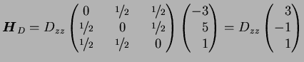 |
(6.8) |
The Fermi contact field,
![]() (Equation 2.18), is much larger (
(Equation 2.18), is much larger (
![]() in DyFe
in DyFe![]() ) and lies along the magnetic easy axis,
) and lies along the magnetic easy axis,
![]() in this case. Vector adding
in this case. Vector adding
![]() and
and
![]() gives the total hyperfine field at the site,
gives the total hyperfine field at the site,
![]() .6.1 The relative magnitude of the quadrupolar interaction can then be calculated using the angle,
.6.1 The relative magnitude of the quadrupolar interaction can then be calculated using the angle, ![]() , between the resultant total hyperfine field,
, between the resultant total hyperfine field,
![]() , and the direction of
, and the direction of ![]() for that site using
for that site using
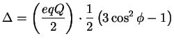 |
(6.10) |
The initial magnitudes of
![]() and
and
![]() are estimates taken from bulk systems. After the spectrum is fitted according to the values obtained as in the above method and the best fit is obtained, the fitting parameters can be analysed. Taking a pair of total hyperfine field values and the known angle between
are estimates taken from bulk systems. After the spectrum is fitted according to the values obtained as in the above method and the best fit is obtained, the fitting parameters can be analysed. Taking a pair of total hyperfine field values and the known angle between
![]() and
and
![]() a simultaneous equation can be used to extract
a simultaneous equation can be used to extract ![]() and
and ![]() . These derived values can then be used to calculate a new set of initial fit parameters and the whole process is repeated in an interative fashion until stable values are obtained.
. These derived values can then be used to calculate a new set of initial fit parameters and the whole process is repeated in an interative fashion until stable values are obtained.
Dr John Bland, 15/03/2003
![$\displaystyle \mathbf{D}_{[111]} = \left( \begin{matrix}
\phantom{-}0 & \phanto...
...nicefrac{1}{2} & \phantom{-}\nicefrac{1}{2} & \phantom{-}0
\end{matrix} \right)$](img509.png)
![$\displaystyle \mathbf{D}_{[11\bar{1}]} = \left( \begin{matrix}
\phantom{-}0 & \...
...{2} \\
-\nicefrac{1}{2} & -\nicefrac{1}{2} & \phantom{-}0
\end{matrix} \right)$](img510.png)
![$\displaystyle \mathbf{D}_{[\bar{1}11]} = \left( \begin{matrix}
\phantom{-}0 & -...
...nicefrac{1}{2} & \phantom{-}\nicefrac{1}{2} & \phantom{-}0
\end{matrix} \right)$](img511.png)
![$\displaystyle \mathbf{D}_{[1\bar{1}1]} = \left( \begin{matrix}
\phantom{-}0 & -...
...hantom{-}\nicefrac{1}{2} & -\nicefrac{1}{2} & \phantom{-}0
\end{matrix} \right)$](img512.png)