Temperature Dependence

A hysteresis curve gives information about a magnetic system by varying the applied field but important information can also be gleaned by varying the temperature. As well as indicating transition temperatures, all of the main groups of magnetic ordering have characteristic temperature/magnetisation curves. These are summarised in Figures 3.7 and 3.8. At all temperatures a diamagnet displays only any magnetisation induced by the applied field and a small, negative susceptibility.

The curve shown for a paramagnet is for one obeying the Curie law,

$$\chi = \frac{C}{T}$$ (3.8)

and so intercepts the axis at $T=0$. This is a subset of the Curie-Weiss law,

$$\chi = \frac{C}{T-\theta}$$ (3.9)

where $\theta$ is a specific temperature for a particular substance (equal to 0 for paramagnets).

Figure 3.7: Variation of reciprocal susceptibility with temperature for: (a) antiferromagnetic, (b) paramagnetic and (c) diamagnetic ordering.

Figure 3.8: Variation of saturation magnetisation below, and reciprocal susceptibility above $T_{c}$ for: (a) ferromagnetic and (b) ferrimagnetic ordering.

Above $T_{N}$ and $T_{c}$ both antiferromagnets and ferromagnets behave as paramagnets with $\nicefrac{1}{\chi}$ linearly proportional to temperature.^3.4 They can be distinguished by their intercept on the temperature axis, $T = \theta$. Ferromagnetics have a large, positive $\theta$, indicative of their strong interactions. For paramagnetics $\theta \cong 0$ and antiferromagnetics have a negative $\theta$.

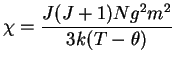
The net magnetic moment per atom can be calculated from the gradient of the straight line graph of $\nicefrac{1}{\chi}$ versus temperature for a paramagnetic ion, rearranging Curie's law to give

$$\mu = \sqrt{\frac{3Ak}{Nx}}$$ (3.10)

where $A$ is the atomic mass, $k$ is Boltzmann's constant, $N$ is the number of atoms per unit volume and $x$ is the gradient.

Ferromagnets below $T_{c}$ display spontaneous magnetisation. Their susceptibility above $T_{c}$ in the paramagnetic region is given by the Curie-Weiss law[10]

$$\chi = \frac{J(J+1)Ng^{2}m^{2}}{3k(T-\theta)}$$ (3.11)

where $g$ is the gyromagnetic constant. In the ferromagnetic phase with $T \lesssim T_{c}$ the magnetisation $M(T)$ can be simplified to a power law, for example the magnetisation as a function of temperature can be given by

$$M(T) \approx \left(T_{c} - T\right)^{\beta}$$ (3.12)

where the term $\beta$ is typically in the region of 0.33 for magnetic ordering in three dimensions.

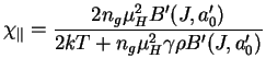
The susceptibility of an antiferromagnet increases to a maximum at $T_{N}$ as temperature is reduced, then decreases again below $T_{N}$. In the presence of crystal anisotropy in the system this change in susceptility depends on the orientation of the spin axes: $\chi_{\parallel}$ decreases with temperature whilst $\chi_{\perp}$ is constant. These can be expressed as

$$\chi_{\perp} = \frac{C}{2\theta}$$ (3.13)

where $C$ is the Curie constant and $\theta$ is the total change in angle of the two sublattice magnetisations away from the spin axis, and

$$\chi_{\parallel} = \frac{2n_{g}\mu_{H}^{2}B^{\prime}(J,a_{0}^{\prime})}{2kT + n_{g}\mu_{H}^{2}\gamma\rho B^{\prime}(J,a_{0}^{\prime})}$$ (3.14)

where $n_{g}$ is the number of magnetic atoms per gramme, $B^{\prime}$ is the derivative of the Brillouin function with respect to its argument $a^{\prime}$, evaluated at $a_{0}^{\prime}$, $\mu_{H}$ is the magnetic moment per atom and $\gamma$ is the molecular field coefficient.